This article is the first of a group of three that will discuss normal-maps and our measurement results compared to common methods proposed which use different softwares and tutorials (nVidia Texture Tool, Gimp, Photoshop, xNormal, AwesomeBump, ….). If you’re familiar with the concept of height-maps and normal-maps, you may still be interested in the two following.

Normal vector

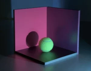
The term “normal” is a mathematical term that means “perpendicular”. A normal vector is a vector perpendicular to the tangent line of a curve in 2D or a to the tangent plane of surface in 3D. The useful informations of a normal vector are its origin on the object and its direction and its norm (= its length) is taken as 1 by convention. In the illustration below, red arrows are normal vectors to the circle or to the ellipsoidal shape.

In the case of image rendering, we’re interested in objects surfaces and the image above illustrates how local normal vectors directions are related to the local shape. The normal vector is used to calculate the angle of incidence of light with the surface which is needed to determine the quantity of light that’s reflected or transmitted in each direction.

Height-map

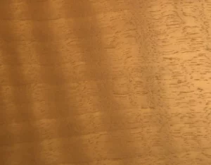
Let’s consider a surface that’s flat in average but with a slightly rough texture. On the illustration below, the color represents the height of the surface from black (minimum height h_min) to white (maximum height h_max). The height is a function of the (x,y) coordinates.

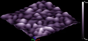
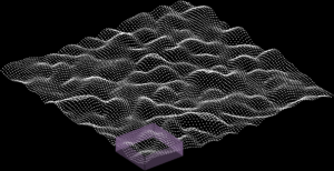
The two steps to obtain a height-map from a given surface are sampling and quantization. The sampling consists of creating a regularly-spaced grid of points in the (x,y) plane and calculating for each point its height value h(x,y). Then, the quantization is the process that transforms these continuous values into a finite set of integer values.

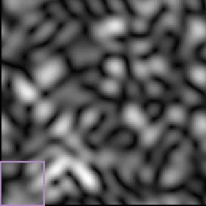
For an 8-bits precision image, only 256 values are permitted from 0 to 255 included. One possible and very straightforward transform from heights h to quantized values Q is the affine transform Q = round(2⁸(h-h_min)/(h_max-h_min)). The images below illustrate the principle of sampling the surface and then displaying the quantized values as a gray-level image. The bottom left of the image corresponds to the bottom corner of the 3D view.

Normal-map

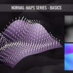
What is sampled to obtain the normal-map of the surface is the coordinates of the normal vectors. The images below shows normal vectors for a gridded sampling of (x,y) coordinate, on the left with their origin are set on the surface and on the right with their origin set on the z=0 plane.

 

At this step, each point of the sampling grid has a corresponding normal vecotr, thus three corresponding normal vectors coordinates. Since typical RGB images have three values per pixel, it would be convenient to asssociate each sampling point to a pixel and each vector coordinates to a color channel value. In the 3D space (x,y,z), the coordinates of a given normal vector v are between -1 and 1 for the v_x and v_y coordinates and between 0 and 1 for the v_z coordinate, whereas RGB values are generally integers between 0 and 2^k-1 for k-bits images (8-bits or 16-bits).

The affine transform C= round(2^k-1(1+v)), where C represents the R, G or B and v the coordinate x, y or z coordinate of the vector, is used for the conversion and the continuous segment [-1;1] is quantized within the integer set from 0 to 2^k-1. To each vector direction corresponds a color which is shown on the video below. Note that some softwares may have other conventions and flip the direction of either the x-axis. Also, since the z coordinate is always positive, half of the dynamics of the B channel is unused.

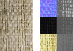
In the case of the surface used in the tutorial, the normal-map is given below. reddish shades corresponds to slopes whose normal vectors have positive x and negative y coordinate, thus pointing downwards right in this convention. Like the height-map, the continuous range of values for the vectors coordinates are quantized on a finite set of 2^k values per channel in the case of k-bits images. Also, since the coordinates of the normal vector must correspond to a norm of 1, not all the colors are possible in a normal-map.

Conclusion

Normal-maps and height-maps are regular sampling of data related to a 3D surface considered flat at a large scale. The sampled values are then transformed into values available in typical images formats using simple conversion formulas. The next article will compare our results which are based on physics with softwares that propose to create normal-maps from materials pictures by making strong assumptions and that obtain questionnable results and the final article will deal with the relationship between the two maps and the impact of quantization on the recorded information.

Our materials are available in different variations. Each of them is optimized for a given type of light source. This guide will help you choose which version to get depending on your needs.

Default choice

If you’re not looking for a specific version of a material that would be optimized for a given situation, we suggest that you use the following settings in the Product filters: Illuminant E, Model type GGX and 8-bit quantization. This variation allows you to download the different parameters maps (base color, albedo, roughness, …) individually as well as compiled and source version of the material.

Why so many variations ?

We perform spectral measurements of the materials. This implies that for PBR, the base color we provide is natively a hyperspectral image: to each pixel corresponds a complete spectrum and not just 3 values as in RGB images. However most renderers cannot process hyperspectral images and we have to compute the conversion from the spectrum to RGB values. To do this, the incident light spectrum must be taken into account since the material colors may change depending on the light source it is lit by.

As an example, the two images below are an example of a spectral rendering of the same material under two different illuminants, namely D65 (daylight) on the left and LED-like spectrum on the right. Even though the white squares appear the same, which also means that the sources themselves have the same color, the colored squares differ more or less in shades.

 

Why is Illuminant E the default version ?

Illuminant E has a flat spectrum, i.e. the same energy emitted at each wavelength over the visible spectrum between 380 nm and 780 nm. Thus, a RGB base color map computed under this illuminant is “neutral” and can be used in RGB rendering with colored light sources (RGB triplet or CCT value) to obtain an acceptable approximation of the reality with a kind of “average” behaviour of the material.

However, the material will not appear on the rendered image exactly as it does in reality with the Illuminant E version. This is due to the spectral nature of light which causes metamerism: two colors can appear identical under a given illuminant and different under another, as shown on the previous image. This is the reason why we adapt the base color maps to typical illuminants in order to minimize the risk of metameric effects.

Minimize metamerism for more realistic rendering

If you are seeking better color accuracy in RGB rendering, we recommend the use of the other variations of the material. MATEREAL currently proposes base color maps adapted for D65 (daylight), A (blackbody radiation at 2856 K) and high-CRI LEDs with different CCTs. They are optimized assuming the light color used in the renderer is a blackbody with the corresponding CCT:

D65 (6500 K)
A (2856 K)
LED (2800 K)
LED (4500 K )
LED (6000 K)
LED (7500 K)

Using these maps with theses light source values guarantee accurate color simuation with our materials while being compatible with non-MATEREAL materials.

Hyperspectral base colors ?

Hyperspectral base color maps will be available in the products catalog soon, either to be used directly in spectral renderers, or to perform pre-processing you may need before using the material in a scene such as computing the base color for another light source (low-pressure sodium vapor lamp, RGB LED, etc.).

Detailed tutorials on the use of MATEREAL materials and on metamerism will be published in the coming weeks.

Model type and quantization ?

Various analytical models exist to approximate materials BRDFs such as GGX and Ward. Both can be used in PBR materials and have their own strengths and weaknesses to be discussed in coming articles. Depending on your preferences and the renderers you use, you can either use GGX or Ward model type.

Quantization is related to PBR accuracy and only 8-bit maps are available at the moment. 16-bit and HDR will be proposed in the coming weeks to improve the PBR accuracy, parrticularly or the base-color and normal-maps.

We propose different types of measurements for different needs. Use our contact form if you have any questions regarding our measurement capabilities.
Section I. presents our measurement capabilities in terms of materials appearance and Section II. presents our tools accurate color calibration of images and renders.

I. Materials optical characterization

BSDF	Specular reflection	Sparkles
Material BRDF and/or BTDF in visible light and in the near-infrared domain.	Radiance ratio in the specular direction as a function of the incidence angle.	Sparkles chartacteristics in glistering materials such as metallic car paints.
high angular precision captures all optical phenomena	from 0° to 90°	sparkle density and angular width histogram
– suits best homogeneous materials – backscattering can be discussed	– homogeneous materials with clearcoat or polished surface – transparent polished materials	– materials with small reflective flakes – colored sparkles can be discussed
Refractive index	Normal-map and models maps	Other specific needs ?
Complex refractive index ñ(λ) = n(λ)+i k(λ)	Normal-map and materials models maps (diffuse, roughness, …).	Please tell us more about your needs and we will discuss solutions.
	resolution up to to 30 µm/pixel XYZ, RGB or spectral base-color, optimized for the illuminant
– for non-translucent materials with parallel polished surfaces	– multiple materials models

 

Coming soon

We are working on various other optical characteristics of mateirals such as the ones presented below.

Diffraction	Polarisation	Anisotropy	Fluorescence	Phosphorescence

II. Color calibration

We also propose different solutions to obtain calibrated XYZ images. More information to come.